How to directly use the Clickhouse DB with Grafana and Collectd

Published: 3.Jul.2020
Last updated: 18.May.2021

Preface

This is a guide about how to set up Collectd to send its data directly to the Clickhouse database and to then use Grafana to display those informations by retrieving them directly from the database, all this while having good performance respectively low resource consumption on all servers that host these components.

This article is very long, which might give you the impression that doing this is very complicated.
It's not! (if you don't have problems setting up those 3 software components)
Most of the stuff I wrote is to explain why I took certain decisions and/or why I set some parameters in a specific way, and to provide at least some examples.

Index

1- Introduction
2- Overview
3- Clickhouse
3a) Download & install and create a database
3b) Tables - overview
3b1) Create the "normal/base" table
3b2) Create the "buffered" table
4- Collectd
4a) Initial URL-builder script
4b) Collectd configuration
5- Grafana
5a) Intro
5b) Macros
5c) SQL examples
5c1) Low difficulty: % used CPU(s)
5c2) Medium difficulty: % free RAM
5c3) High difficulty: written bytes (disk)
6- Results & remarks
7- Downloads
8- Changelog

1- Introduction

I have a a server & some VMs running some services (this website, Nextcloud, email, etc...) => I therefore have to keep an eye on the current consumption of resources (CPU/RAM/disks/...), on the activities performed by some processes (Apache, MariaDB, this website's load time, etc...). Additionally, a chart that shows how those informations changed/evolved over time is often very useful to see if any change done in the past had some indirect repercussion (e.g. a tiny but constant increase CPU usage).
To do that I used so far the following components:

Collectd: to gather metric data about my server/VMs/processes and to forward all that to my database.
Carbon-cache & Carbon/Graphite (with its "Whisper" DB) & Graphite-web: to receive the metric data sent by Collectd, process it, store it and finally to make the data/results available to be queried.
Grafana: to present the data stored in the database by querying Graphite-web.

Having to use/manage all these components hasn't been complicated nor time-consuming, but it did annoy me to have to use "carbon-cache" and "graphite-web" because I felt like that they were superfluous. Additionally, when querying a range higher than 3-4 weeks I often got timeouts in Grafana's charts and the CPU usage on my server was high.
I had a feeling that things could be done in a better way, therefore I started wondering about how to at least get rid of the Graphite components.

The Change:

Having had during the last ~2 years very positive experiences with the database "Clickhouse" (relatively new but stable for me, easy to manage and incredibly fast) I decided to try to replace all the Carbon/Graphite stack with that DB => the end-result had therefore to be:

Collectd: gather metric data and forward it to Clickhouse.
Clickhouse: get + store + serve that data.
Grafana: retrieve the data from Clickhouse and show/present it.

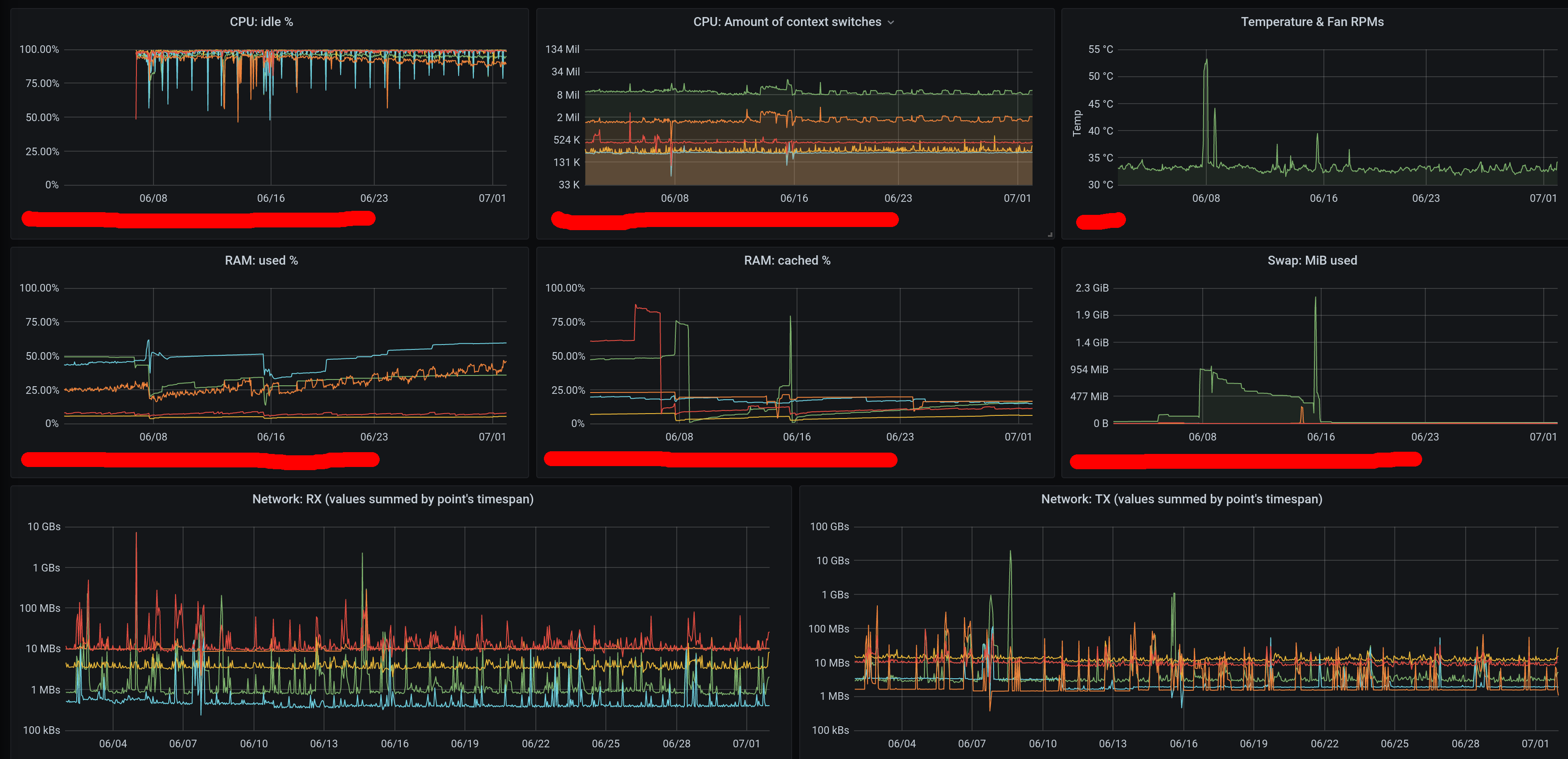
Does it work?
Yes, here it is:
Picture of my dashboard

How's the performance?
Excellent so far, but as of today the DB's data covers only 4 weeks => I'll have to do more tests in the future using more data (I'll post here updates if needed), but I don't expect big surprises.
Actually, let me rephrase that:
the current performance already greatly surpasses (and uses less CPU & disk space & disk I/O than) the one that I had when using Graphite - I don't expect this setup to become slower when even more data will be added, but if that will happen then fixing it will hopefully be trivial (e.g. by modifying the DB's storage parameters or forcing a manual "merge" of multiple DB-"parts" that might lying around, but, based on my personal experience with another private project that used a Clickhouse-DB that contained ~36 billion rows this is unlikely to happen if monitoring just a few thousand combinations of hosts/VMs/metrics).

Advantages? (compared to the previous setup)
1) Less software-components, 2) less used storage space & I/O and 3) faster queries & less CPU usage.

Disadvantages?
None so far.
I'm currently not using in Clickhouse any kind of data pre/post-aggregation mechanism (in my previous setup Graphite used to reduce the resolution of datapoints older than 1 month from 30 seconds to 2 minutes by averaging them), so you could consider this a disadvantage (of my personal implementation; Carbon/Graphite-like aggregation can be done in Clickhouse by modifying the table definition shown below) but on the other hand in my opinion Clickhouse is able to deal with unaggregated data without being slower or using more resources (compared to Carbon/Graphite) therefore the ability to drill down to the original datapoints makes it for me one of those rare win-win solutions with no downsides.

If you decided to do something similar, and are looking for inspiration or are having some problems (maybe not directly related to such an implementation), then hopefully this article will provide some hints :)

Please at least skim through the whole article before starting to fiddle around with your system - maybe some details will be a no-go for you!

You can use this site's "Contact"-link (in the menu at the top) if you have any questions/remarks - I'll give my best to reply, or maybe not if I'm overwhelmed by spam, we'll see.

I wrote a lot to try to explain things as well as possible, which makes the whole thing look extremely complicated => I admit that there are many details to be aware of (most of them have to do with Clickhouse - irrelevent for you if you already understand how that special DB operates), but in the end it's not complicated - I tried to add explanations about why I took certain decisions to give you a good foundation to then in turn be able to take informed decisions for your own personal usecase.

2- Overview

As of today (June 2020), Collectd doesn't have a dedicated "write"-plugin for Clickhouse.
It does have a "write_graphite"-plugin, and Clickhouse has some mechanisms/software to accept data in a "Graphite"-format, process it and make it available (components available in GitHub - unknown to me if they're supported by Clickhouse itself), but I am not using all that because, as I mentioned above, I want to have a "minimal/pure" software architecture.

My solution is as follows:

Collectd uses the "write_http"-plugin to send data directly to Clickhouse.
Clickhouse can accept data through HTTP as part of its standard functionality, therefore Collectd becomes just a normal&standard data feed.
Warning:
the http-URL used by Collectd will contain the cleartext userID&password of the DB (e.g. "http://myuser:mypwd@my_db_server:8123/blahblah..."), therefore you must protect it when the connection is made between physical hosts! (use an ssh-tunnel, a VPN, etc..).
In my case I don't consider this a problem as I would anyway never ever make the DB accessible directly from outside the host, and the Clickhouse-logs (which might log the URL if something goes wrong) are not exported anywhere nor read/analyzed by anything (for the time being => I will have to handle them in a secure way in the future when I'll start to monitor them).
Clickhouse receives "text strings" from Collectd, it splits the strings on-the-fly into their individual components (e.g. hostname, metric name, etc...) and stores each one in its own table-column.
(this mechanism uses the "input" table-function; not sure since which version it's available but at least since version 20.4.2.9 as it's the one that I'm using while writing this)
Grafana uses the Clickhouse DB as datasource directly.
(possible since Grafana 4.6 by using the "Clickhouse datasource" plugin)

The tricky parts were:

Make Clickhouse store the strings that were fed by Collectd over HTTP by separating the fields correctly before writing anything into the DB (the value of each field is then saved directly in its own table column).
(therefore, if you were wondering, I'm not using any kind of "materialized column")
Write in Grafana queries which display the data correctly and which perform the aggregation (when the graph on the screen doesn't have enough width to display each single data point in its own pixel) in the Clickhouse DB (and not in Grafana's server component, as Clickhouse is a loooot more efficient when performing such tasks).

3- Clickhouse

The Clickhouse database can be extremely fast without having to use any special hardware, using at the same time as well less storage (space and I/O) than other DBs:
this can be achieved because it stores data physically "by column" and not "by row" as other classic DBs do (e.g. Oracle, Postgres, MariaDB, etc...), because it uses CPU-features ("SSE 4.2" as of June 2020) to perform certain tasks, and especially because of its pecular way of handling inserted rows: once rows are grouped into a so-called "part" (a part is a "chunk of data", not a "partition) they're all pre-sorted, indexed (a high-level index which basically states if a certain row is potentially present in a specific subset of a "part") and compressed (compressing single "columns" is a lot more efficient than doing the same on "groups of rows" even if the informations handled by the two approaches are identical in both cases).

Of course there is always a price to pay (e.g. in the case of Clickhouse no "transactions", no direct deletions of rows nor any "updates" to values, performance when not querying ranges of rows is worse than classic DBs, joins might be automatically aborted because hitting max temporary RAM consumption thresholds, etc...) but in this case all limitations are irrelevant (metric data does not change, partitions are a good solution to delete old data, queries always access a large amount of data, queries are written to perform data aggregation during the 1st/lowest execution stage, etc...).
Please read the official docs to know more about it.

The settings that you use for both the DB and for the tables have a MASSIVE impact on performance (which can range from "stellar" to "catastrophic") => if performance is bad (but the usecase does fit Clickhouse) then usually it's just your own fault :)

As of June 2020 I like the Clickhouse DB because:

the documentation is good.
(and I liked as well the the code that I saw on GitHub while skimming through it in 2019 and the replies&reactions that I got after submitting issues&questions)
it doesn't require any uncommon SW/HW-components to make it work and it works fine as well with low system specs.
The excellent performance when using spinning disks (HDDs) is for me one one of the key features.
(the DB writes data in its "parts"/"files" always sequentially, with all data ordered perfectly => read-requests can be executed later with sequential I/O per "part"/"file" => not a lot of time wasted by HDD-"seeks" => CoW-filesystems like ZFS used in combination with Clickhouse should therefore deliver as well good performance, which might not be the case when used in combination with classic DBs)
(if using ZFS, I got the best performance when using a "recordsize" of 1-2MiBs)
(using low-specs SSDs and/or an SSD-write-cache might be a bad idea with Clickhouse => it might manage to quickly wear out your SSD, and it's not really needed)
it can be used by many DB/SQL-clients (you'll just have to install its JDBC-drivers).
I use DBeaver and it works perfectly with it as long as I set the "compression"-option to "false" in the driver's connection settings.
Being able to query the DB directly by using SQL adds a lot of flexibility compared to other DBs specialized in big storage that cannot do this, or at least not without another middle-layer <e.g. Cloudera-something in the case of Hadoop/Kobo/etc..., forgot how that's called> which in turn adds complexity.
When trying out a new DB one of my first tests is always to overload the DB and observe how it reacts.
For example when I did this with Apache Kobo & Cassandra, both crashed.
In the case of Clickhouse it started rejecting requests, but it did not crash => this is the minimal type of behaviour I was looking for.
it's reaaally fast.

3a) Download & install and create a database

In my case I created a VM (I'm a fan of " Gentoo Linux" but I'm running Clickhouse in "Linux Mint" VMs just because I like Mint and updates are easier to handle than in Gentoo), I installed the DB in there (as described in the docs of Clickhouse) and I set Clickhouse up to run as a non-prileged user (maybe that was anyway the default of the distro).
I then doublechecked that the host's firewall rules were already blocking all external traffic related to the ports on which Clickhouse is listening ("netstat -tanp | grep LISTEN | grep -i click") and that they let only intra-VMs traffic through.
I created in the Clickhouse-DB a brand new user which is the one that is used by "Collectd" to send metric data to the DB (pls. refer to the official docs) and which has access only to that specific DB.
I will restrict that user's permissions to be able to only insert data into the Clickhouse-table which stores all metric data (this is apparently a new feature in recent versions of the DB but which I didn't manage to use so far).
I'm currently using the same user as well in Grafana to read data from the DB, but I'll soon create an additional read-only user for that so that there will be no big repercussions if that user is somehow compromised.

3b) Tables - overview

In general, 2 tables are needed:

a base/normal table of type "MergeTree" which ultimately stores all data that is received by the "Collectd"-agents.
a table of type "buffered" to receive all incoming data, accumulate all that stuff in RAM for a few seconds/minutes, and then finally flush it at ~regular intervals into the base/normal table.

Reason:
Clickhouse hates many small "inserts"; performance will be terrible and/or I/O rates will be very high if you try to do that (e.g. max from ~1000 ~10000 rows inserted per second depending on your HW, generating a lot of I/O activity) - it would be like using a truck to do pizza-delivery (you can do it, but it's potentially extremely inefficient).
To go towards "millions+" of inserts per second (and to lower the system's resource usage) the DB-creators recommend to pre-aggregate "inserts" and to submit them all using a single SQL.
I did initially ignore that recommendation (of course: "bulls**t - I'll do it my way"), but I admit that I was totally wrong.

As a pre-aggregation is sometimes not possible (in this specific case on one hand the "write_http"-plugin of the Collectd-agent will buffer autonomously some rows before transmitting them, but on the other hand you might as well have many Collectd-agents running on many hosts/VMs all trying to send separately few groups of rows to the DB), the DB itself provides an embedded mechanism to aggregate those inserts => that mechanism is a table of type "buffered":
a "buffered" table sits on top of a real table, mirrors exactly&automatically the structure of its "base"-table, accumulates all incoming rows in RAM and once a certain threshold (defined by you) has been reached it flushes all the rows that it has accumulated into the real physical/real/base table => one (or at most few) I/O can put a looot of rows (hundreds of thousands) into the base/real/physical table.

Here are all the details about both tables:

3b1) Create the "normal"/base table
Here is the definition of the base table that I'm using => this is the table that physically saves the data in your filesystem (ext4, ZFS, XFS, etc...):

create table collectd_metrics
(
host String CODEC(ZSTD(1))
,item String CODEC(ZSTD(1))
,measurement String CODEC(ZSTD(1))
,m_interval UInt32 CODEC(ZSTD(1))
,m_timestamp DateTime CODEC(Delta, ZSTD(1))
,val1 Double CODEC(Delta, ZSTD(6))
,val2 Double CODEC(Delta, ZSTD(6))
)
engine=MergeTree()
PARTITION BY toYear(m_timestamp)
order by (measurement, item, host, m_timestamp)
settings index_granularity=32768,min_merge_bytes_to_use_direct_io=999999999999999999

The first section of the SQL, which defines the columns, mirrors the informations sent (respectively the hierarchy set) by Collectd, over HTTP.
Here is an example of a string sent by Collectd for a single datapoint (more precisely this is a datapoint having 2 dimensions, which can happen depending on the type of metric - more infos in the "Collectd"-chapter):

PUTVAL my_hostname/interface-eth0/if_octets interval=30.000 1590962489.447:1178454697:4762592275

When data arrives I discard the "PUTVAL" string (useless as always present in all rows) and sub(&sub)-string the rest (all detailed infos available in the chapter about "Collectd").
The next substring (in this example "my_hostname/interface-br0/if_octets") is split as follows:

the first value ("my_hostname") is always the hostname set by the Collectd-agent which runs on each individual host/VM ("host" in my table).
the second one ("interface-eth0") is "which device is being monitored on that host" ("item" in my table - can be a network card, a disk, a CPU, etc...).
the third one ("if_octets") is "which device parameter is being monitored" ("measurement" in my table).

Up to you if to use the same names or better ones (I admit that both "item" and "measurement" are not optimal but I wanted to keep things generic as I wasn't sure about Collectd's structure - some metrics that you're monitoring through some Collectd-plugins might not comply to this kind of standard).

The column "m_interval" contains whatever comes after the equal-char of the substring "interval=30.000".
(in my case I set Collectd wth an interval of 30 seconds for all metrics on all monitored hosts)
(prefixed with "m_" to avoid conflicts in the DB with the existing datatype that has the same name)
(using "UInt32" and not e.g. "float" as I'm sure that I'll never ever set any interval to be a fraction of a second)
(I'm not using that value for anything in Grafana's SQLs, but you could => up to you)

The last substring ("1590962489.447:1178454697:4762592275") is then sub-stringed into its individual parts (split by the "colon"-character (":")):

the first value is the timestamp ("m_timestamp" in my table).
(it's the Unix "epoch", if I remember correctly)
(prefixed with "m_" to avoid conflicts with the existing DB-datatype)
the second and third value are the values of the metric, respectively of what is being measured ("val1" and "val2" in my table).
This is a little bit tricky as many metrics have only the 1st value (e.g. "uptime"/"CPU usage"/"number of processes"/etc... can have only 1 value).
Metrics which have 2 values are for example the ones that have both input&output, therefore e.g. network devices (bytes read & written), disks (bytes read & written), etc... .

The second section of the SQL is all about the parameters of the table.
It is extremely important and, indirectly, it's as well related to the "codec"-instructions of the single columns of the previous block.
Here are some comments related to its individual sections:

engine=MergeTree()
As I mentioned above I'm not using the GraphiteMergeTree table engine because I hope that Clickhouse manages to deliver excellent performance when dealing with non-aggregated data.
The "MergeTree"-table is "the" standard table-type in Clickouse.
-
Infos about Clickhouse itself are not really part of this guide (better if your read the docs on the official website), but just to summarize:
the standard "MergeTree" table engine is basically a hierarchical-aggregating engine where a "bundle" of incoming data is written (sorted by your "order by"-clause & split by column & compressed by column) into a "part", then the next bundle is as well written into its own part, and so on, and once there are a certain amount of parts, they're all read and merged together into a single bigger part of a higher level => then the the whole thing starts over again, until there are once more many low-level parts, which are then all aggregated into a single "higher" part, and so on => when there are many higher parts, they're all once more read and merged into a single part of an even higher level, and so on.
-
The "parts" which are not used anymore, respectively which were read to merge their data into a new big part of a higher level, will stay around for a while just in case that you have a catastrophic failure and that the higher-level-part that was just created is lost/corrupted by your HW => set in the DB's config a limit of something like 5-10 minutes for them (parameter "old_parts_lifetime"), long enough to be at least 100% sure that that the OS and the HW that you're using will by then have flushed all dirty buffers to the lowest HW-devices and that the lowest HW-device's cache will have written all cached data to the physical medium (but on the other hand don't set that parm too high to avoid to clog your filesystem with too many files).
PARTITION BY toYear(metric_datetime)
It's usually a bad idea to use partitions in Clickhouse (I keep falling into this trap) as it's totally different from a normal DB.
As Clickhouse splits/aggregates data into "parts" (again, not a "partition" - similar to it as it's nicely sorted and compressed, but it does not have predetermined physical boundaries), and as each "part" with this table structure creates in this specifc case ~20 files, having "partitions" which would forcefully create additional sets of files would decrease performance when querying the data (many file-handles to open/close, less efficient indexing and compression).
In my case this is no exception:
partitioning the table on a level lower than by year (e.g. by month is the usual recommendation) is very likely to lead to a decrease of performance (or depending on your point of view, to an increase of resource consumption) as soon as the timerange that I would query would involve more than 1 month, while partitioning by year would only lead to more storage being used (as, compared to partitions that would be dedicated to single months, I will not be able to immediately drop single partitions of months that are older than 2 years).
-
Really: forget "partitioning" if you did like it when using classical DBs.
Clickhouse keeps (re)creating "parts" from scratch, therefore there is no danger of data getting entangled/mixed.
When querying data, even if you end up having a single "part" of 20TiB, Clickhouse won't just scan it blindly but it will first do a lookup in the index of that "part" to know which "chunks" of the part will have to be checked (the amount of rows which define a "chunk" of data in a "part" is defined by the parameter "index_granularity", please see below) and it will therefore use resources to only access those few bytes of data.
order by (measurement, item, host, m_timestamp))
This parameter is crucial: it will have an impact on everything, from the final performance of the queries to the CPU & RAM & I/O usage on your server.
It sets how the data will be physically sorted in the table (in each individual "part" that will make up a partition).

It might be the opposite of what you're expecting (if you were expecting e.g. the timestamp to be in the first position, and then maybe as well the rest to have the same hierarchical order used by the table columns definition).

The reasons to sort rows like this are that...
1)
this offers the absolutely best compression (great compression with minimal cost) as all values that are related to each other will be sequential (perfectly "near" each other) and finally ordered sequentially by timestamp (their values will therefore change only slightly row-by-row).
2)
when querying a relatively large range of data, all datapoints related to each other will be in the same block or at least in sequential blocks (potentially in the same file/"part", depending on how many "parts" you'll have), which in turn will offer great performance on normal HDDs (sequential reads are their greatest friends) respectively low resource consumption.
Therefore, by using this sorting, in a "part" (sorted chunk of rows) most values of "measurement" like "item" and "host" will all be the same/repeated, offering therefore the best performance during both de/compression.
Additionally, most values of "val1" and "val2" might change only slowly value-by-value (e.g. "uptime" will have constant identical increases, unless the host/VM is rebooted), offering therefore as well in those columns additional benefits when de/compressing them (that's the reason why I'm using the "Delta" algo in those column definitions before that the final zstd-compression is applied ).

The other very important reason why I'm putting the "measurement" at 1st place is because it will be the most likely "where-clause" that will be included in my queries.
E.g. I might create a dashboard that shows for many hosts (therefore no selectivity on the "host" column) the amounts of bytes read from multiple disks => in this case the only selection guaranteed 100% will be "amount of bytes" (column "measurement") while both "host" (many hosts) and "item" (many disks) will be undefined or fuzzy => only an index using "measurement" in its first position will guarantee maximum elimination of what the query does not want to know.

This is related as well to the "CODEC"-instructions of the single columns:
as with this column-order each column gets so many sequentially repeated values, the first level of zstd-compression is more than enough to reach a fantastic level of compression (higher levels might make you use more CPU and disk space => pls. test it if you don't believe this).
The only columns which might be challenging are "val1" and "val2", as they contain the real measurements, which is why I 1) run the "Delta"-algo against them to maybe see if they vary maybe by always a small amount and then 2) compress all deltas with zstd level 6 which is not weak but not too hard on a relatively modern CPU.
settings index_granularity=32768,min_merge_bytes_to_use_direct_io=999999999999999999
"index_granularity" specifies how detailed the "index" of the table should be, respectively, how many rows a single index-entry should represent (most probably as well how much data a block/chunk should contain, which will in turn impact compression ratios, as the larger the block the more successful compression might be).
If you don't specify "index_granularity" then Clickhouse will set it to its default which is I think 8192.

As with the order mentioned above ("measurement, item, host") each single measurement will be nicely ordered by the single metric that you'll monitor, you can compute the value that you'll need.
In my case each single metric will be sampled by Collectd every 30 seconds => the default value of 8192 rows-per-index-entry would therefore hold ~3 days (8192*30/60/60/24) worth of data, but 32768 will hold 4 times as much being ~11 days (32768*30/60/60/24) => as I'll likely query data ranges spanning over more than a week a granularity of 32768 makes most sense to me (a higher value will lead to better compression, but worse performance when querying smaller timeranges => up to you).

"min_merge_bytes_to_use_direct_io":
recent versions of Clickhouse should recognize automatically if a filesystem supports directI/O.
I started using partially ZFSonLinux in 2019 and at that time this wasn't the case (which lead to very weird problems), therefore I'm still using this workaround now to be 200% sure that nothing will ever break => up to you (leave it out if you use a filesystem that supports directI/O like e.g. ext4).

3b2) Create the "buffered" table

Now that the "base/real/physical" table exists the "buffered" table can be created.
Here we go:

create table collectd_metrics_buffered as collectd_metrics
engine=Buffer(health_metrics,collectd_metrics,8, 60,120, 100000,1000000, 52428800,104857600)

This creates a fake table named "collectd_metrics_buffered" on top of the real/base-table "collectd_metrics" located in the database "health_metrics".
Why to I have to specify twice the real/physical table? No clue, but so far this way it always worked fine - if you know then please let me know :)
The line...
engine=Buffer(health_metrics,collectd_metrics,8, 60,120, 100000,1000000, 52428800,104857600)
...sets minimum&maximum limits of when it is supposed to flush into the real/physical table the data that it has gathered in RAM:

if all minimum limits are reached, the contentes of the buffer-table will be flushed into the real/physical/base one.
if at least 1 maximum limit is reached the same will happen.

The parameters "...,8, 60,120, 100000,1000000, 52428800,104857600" have the following meaning:

"8": amount of parallel threads to be used for this buffered table.
An incoming row (in this case the single ones generated by Collectd) will be hashed and will be inserted randomly into one of these threads.
Each thread is independent from the other ones and the limits that are set are checked independently on a thread-level => therefore, if you set in these parms a limit of 100MiB then you'll have to multiply that by 8 to know how much total RAM you'll end up needing in the worst case.
I used in the past 16 such threads for hardcore insert jobs (~100'000 rows/s? Cannot recall anymore but it was a lot) therefore in this context 8 are probably overkill for a few hundred rows/s (I see some disadvantages at having more if not monitoring more than at least maybe ~20-30 hosts/VMs, but it probably depends as well on which and how many metrics you're monitoring => it could be that when having a low amount of incoming data less threads will lead to less I/O with no downsides => please play with it!).
"60,120": minimum and maximum time that rows should be buffered without being flushed to the base/real table.
"100000,1000000": minimum and maximum amount of rows to be buffered without being flushed to the base/real table.
"52428800,104857600": minimum and maximum amount of bytes to be buffered without being flushed to the base/real table.

I my case I looked at the string...
PUTVAL my_host/interface-eth0/if_octets interval=30.000 1590962489.447:1178454697:4762592275
....and saw that it's 92 bytes long (ascii) => let's consider a worst-case-scenario and set that to more than 4 times as much (e.g. long hostnames that include the domain, non-ascii chars, etc...) being ~400 bytes:
I have 1 physical host and 4 VMs running on it, which means 5 Collectd agents sending similar streams to the DB, and during each cycle (30 seconds) there are more or less 1150 different metrics ("select count(distinct host, item, measurement) from collectd_metrics") sent to the DB from each host => as each one would need ~400 bytes then the DB would get ~460KiB every 30 seconds.

Having set the limits as shown above, I'm therefore sure that that the only primary driver that triggers the flush of that buffer to disk will be the maximum time:
I feel comfortable to potentially lose max 120 seconds worth of data if my VM/hypervisor/host crash, but not more than that (as those metrics might give me a hint of what was happening shortly before that crash, e.g. 100% RAM usage, swapping, etc...).
Setting a lower max time would be an option for you if your disk subsystem has capacity and won't be consumed by it.
Setting a higher max time (and maybe as well max parameters for the other limits) would be an option if e.g. your Clickhouse DB is running on a separate physical host in a different location (therefore minimal chances that it would end up having the same potential problem(s) experienced by the hosts/VMs that are being monitored).

Fyi:

when you "drop" the "buffered"-table, the rows won't be lost but they'll all be immediately flushed to the base table (and then the buffered-table will be dropped, but it won't otherwise have any other effect on the base/real table).
the "buffer"-table will be used as well by Grafana when reading/querying data (you'll get the most up-to-date result composed of what is stored in the physical/normal/base table and what is stored temporarily in the "buffer" table).

4- Collectd

As I mentioned at the top, one of the major challenges was to make the Clickhouse DB put the informations delivered by Collectd into the right table-columns without first writing anything anywhere.
Here are my 2 examples of what kind of data can typically be delivered by Collectd:

PUTVAL my_megahost/interface-br0/if_octets interval=30.000 1590962489.447:1178454697:4762592275
PUTVAL my_littlevm/apache-apache80/apache_bytes interval=30.000 1590867731.276:12653568

My first attempt was (of course) to use a single "real" column to store the original string received by Collectd and to then split it into its single values by using materialized columns.
It was inelegant to do that, but at that time I didn't care too much, and it did work, but in the end I had to admit that it was using a looot more storage than I expected (at least 3 times more than now), and that coupled with the fact that the solution was "dirty" made me feel uncomfortable.

I then took a step back and tried again to find informations about splitting the incoming Collectd-strings into single columns before writing anything anywhere, and while scanning all Clickhouse's docs I finally came accross the "input" function (doc URL above) which allowed me to do exacly that.
Unluckily, as far as I understood (and I might be wrong), the "input"-function is not something that can be defined in the DB itself but it must be explicitly used when I trying to insert data into Clickhouse => this means that the URL used by Collectd to push data into Clickhouse has to specify not only stuff like the target table but as well the exact instructions about how to split the long Collectd-string(s) into its individual substrings that fit each target table column, which in turn makes the URL quite long and complicated => it is a problem, but it can be managed with a bit of determination, yo :)

4a) Initial URL-builder script

(if you used the same table structure that I used above then you can skip this and just use the URL that I posted in the next chapter)

What you need is a URL which tells the Clickhouse-DB to split in a certain way the strings delivered by Collectd by using the "input"-function.
The task is simple but the exact instructions, when included as part of a URL, can become quite long and messy.

To handle the complexity of writing a long URL I wrote a very simple script to break that into individual lines & sections.
You can of course write the final URL directly on the fly but I personally liked more this approach (I had a bug in the timestamp-column and this script allowed me to identify it easily).
(not really a script - it mostly just concatenates strings)
Here it is (please customize it if you used a different table name and/or column data types):

#!/bin/bash

URL="http://db_userid:db_user_pwd@db_hostname:8123/?query="
URL="$URL INSERT INTO health_metrics.collectd_metrics_buffered SELECT"

#host
URL="$URL splitByChar('/', splitByChar(' ', orig_msg)[2])[1]"
#item
URL="$URL ,splitByChar('/', splitByChar(' ', orig_msg)[2])[2]"
#measurement
URL="$URL ,arrayStringConcat(arraySlice(splitByChar('/', splitByChar(' ', orig_msg)[2]), 3), '/')"
#m_interval
URL="$URL ,toUInt32(cast(replaceOne(splitByChar(' ', orig_msg)[3], 'interval=', '') as Double))"
#m_timestamp
URL="$URL ,toDateTime(toUInt64(cast(splitByChar(':', splitByChar(' ', orig_msg)[4])[1] as Double)))"
#val1
URL="$URL ,cast("
URL="$URL splitByChar(':', splitByChar(' ', orig_msg)[4])[2]"
URL="$URL as Double)"
#val2
URL="$URL ,cast("
URL="$URL if("
URL="$URL length(splitByChar(':', orig_msg)) > 2"
URL="$URL ,splitByChar(':', splitByChar(' ', orig_msg)[4])[3]"
URL="$URL ,'0.0'"
URL="$URL )"
URL="$URL as Double)"

URL="$URL from input('orig_msg String')"
URL="$URL FORMAT CSV"

URL_CONVERTED=$(echo "$URL" | sed 's/ /%20/g')
echo $URL_CONVERTED

#cat input.txt \
#   | curl \
#   "$URL_CONVERTED" --data-binary @-

At the end the script takes the contents of the variable "URL" (which contains the very-long-human-readable-URL) and replaces all ascii-"spaces" by "%20" => the output of "echo $URL_CONVERTED" will then show you the final URL that you'll have to use.

Test the execution of the above script and if everything goes well (no typos) then create an "input.txt" containing at least the following (2 rows/metrics, one with one dimension, the other one with two dimensions):

PUTVAL ultrahost/interface-br0/if_octets interval=30.000 1590962489.447:1178454697:4762592275
PUTVAL tinywebvm/apache-apache80/apache_bytes interval=30.000 1590867731.276:12653568

After having executed the above script while having the last 3 rows uncommented, a "select * from health_metrics.collectd_metrics_buffered" should show in your DB-client the 2 matching rows - congratulations :)
If that's not the case then check 1) the output of the script and 2) the output of Clickhouse (e.g. "/var/log/clickhouse-server/clickhouse-server.log", which is usually very verbose).

4b) Collectd configuration

Assuming that the above test worked, you can copy the looong URL that was generated by the little script and put it into your Collectd.conf-file:

LoadPlugin write_http
<Plugin "write_http">
   <Node "example">
      URL "http://db_user:db_user_pwd@db_hostname:8123/?query=%20INSERT%20INTO%20health_metrics.collectd_metrics_buffered%20SELECT%20splitByChar('/',%20splitByChar('%20',%20orig_msg)[2])[1]%20,splitByChar('/',%20splitByChar('%20',%20orig_msg)[2])[2]%20,arrayStringConcat(arraySlice(splitByChar('/',%20splitByChar('%20',%20orig_msg)[2]),%203),%20'/')%20,toUInt32(cast(replaceOne(splitByChar('%20',%20orig_msg)[3],%20'interval=',%20'')%20as%20Double))%20,toDateTime(toUInt64(cast(splitByChar(':',%20splitByChar('%20',%20orig_msg)[4])[1]%20as%20Double)))%20,cast(%20splitByChar(':',%20splitByChar('%20',%20orig_msg)[4])[2]%20as%20Double)%20,cast(%20if(%20length(splitByChar(':',%20orig_msg))%20>%202%20,splitByChar(':',%20splitByChar('%20',%20orig_msg)[4])[3]%20,'0.0'%20)%20as%20Double)%20from%20input('orig_msg%20String')%20FORMAT%20CSV"
   </Node>
</Plugin>

(Re)start your Collectd daemon, keep your fingers crossed, wait for a few seconds and check both the logs of Collectd & Clickhouse.
If you don't see any warning/error message then execute "select * from health_metrics.collectd_metrics_buffered" and the new Collectd data should show up after a few seconds => if you do see the data then congratulations, you did it :)

5- Grafana

At this stage the metric data is being gathered by Collectd, forwarded to the Clickhouse DB and stored in there.
The only thing that is left to do is to display that data graphically.

As I mentioned at the beginning of the article: download & install Grafana's Clickhouse-plugin, then in Grafana configure it so that the the plugin confirms that it can connect to the Clickhouse DB.
Finally create in Grafana a new dashboard and add a panel (a chart).
The next sections will focus on configuring the panels depending on the type of data that is being queried (stick with a normal chart until it works, as it makes debugging a lot easier - once that works you can format it in any way you want).

5a) Intro

The database will end up hosting millions of datapoints for each metric - for example in my case each metric is measured once every 30 seconds, therefore a timespan of 2 years will hold ~2M rows for each metric => the DB itself will not be impressed by this amount of data, but Grafana&your browser definitely will be (which would result in hangs/crashes) if you try to forward them all that data.

The absolutely crucial thing when writing queries in Grafana is therefore to perform the aggregation in the DB itself, before that any data is sent from the DB to Grafana.
The aggregation done in the DB is supposed to restrict the amount of rows of the result sent to Grafana to the amount of horizontal pixels that can be used by the chart shown in your browser (you cannot display/plot more datapoints in the chart than the amount of pixels that you have available => anything more than that would just put more load on your CPU&RAM with no benefits).

To restrict the amount of rows sent from the DB to Grafana you'll therefore have perform some sort of aggregation => you can decide on your own if to use an avg, max, min, etc... depending on the information that you want to show in the charts and your own way of thinking.

Most of the complications mentioned below are related to those aggregations.

Concerning Grafana itself, I'm not a pro at using it => I don't use clever functionalities like variables, dropdown-menus, etc..., so up to you to make things fancy if you are able to and have a need for them.

5b) Macros

The Clickhouse-plugin for Grafana provides some very useful "macros" that can be used in the SQLs that are executed against the DB to retrieve the needed data: they generate parts of an SQL depending on which parameters and other stuff is being used by Grafana when the data is queried (e.g. the timerange that is selected, the physical size of the chart displayed in your browser, etc...).
The (only) ones that I keep using in my SQLs are:

$table
Very simple: it is replaced by the from-clause for the source table that you're using.
Example: "FROM health_metrics.collectd_metrics_buffered"
$timeFilter
As well very simple: it is replaced by a where-condition that selects the timerange of the data that you are querying in Grafana
Example: "WHERE m_timestamp >= toDateTime(1593273217)"
$timeSeries
Extremely important: it performs an aggregation of the rows in the DB based on the timerange that you're querying and the amount of space that you have on screen to display the results and (optionally) the "resolution"-parameter that you set in the properties of your charts.
Example: "(intDiv(toUInt32(m_timestamp), 60) * 60) * 1000".
If you'll increase the queried timerange or decrease the width of your window then you should see that the values "60) * 60)" will increase (to e.g. 120 or 300, etc...) => as you have the same space available to display more data (bigger timespan) or have less screen area to display the same data (shrunken width) the DB will have to increase the level of data aggregation to generate less datapoints compared to the original resolution of informations that are available in the DB.

Based on what I mentioned in the "intro", the "$timeSeries"-macro is therefore the key to keep resource usage low everywhere when refreshing the chart contents => it must therefore be executed as early as possible in the DB (if not then you will have bad performance and/or run out of RAM on your VM), and that is one of the challenges when writing in Grafana the SQLs that retrieve the needed data.

5c) SQL examples

Here are the explanations about how to write the SQLs for the most common usecases.
They might not be absolutely perfect, but they should demonstrate technically what I meant in all my previous remarks.
All the SQLs used by my own dashboard can be downloaded in the "downloads"-chapter below.

5c1) Low difficulty: % of total used CPU(s)

I assume that you have this in your Collectd.conf:

<Plugin cpu>
        ReportByCpu false
        ValuesPercentage true
</Plugin>

(the values sent by Collectd will represent, as a percentage, how much all CPUs were in some state during the whole timespan of the Collectd cycle, which in my case is 30 seconds)

This is valid for all charts:
ensure that you're not in the "SQL edit mode" (if you are then click on the small "pen"-icon to get out of it) and set the values for...
"-- database --" & "-- table --" & "-- dateTime:col --"
...to...
"health_metrics" & "collectd_metrics_buffered" & "m_timestamp"
... and of course adapt this if you used other names in the table definition.

Then change to the "SQL edit mode" and paste this query:

SELECT
    $timeSeries as t, host, min(val1 / 100)
FROM $table
WHERE
    $timeFilter
    and item = 'cpu'
    and measurement = 'percent-idle'
GROUP BY
    host,t
ORDER BY
    host,t

Refresh the chart (in Linux & Firefox I can just press ctrl+enter when the cursor is the SQL-editor) and you should see the results (the amount of CPU which was idle) plotted in the chart for all hosts that you're monitoring.
If you don't see anything then click on "Query inspector" to see if the DB returned any error message.
To then do deep debugging of the query click on "Generated SQL", copy the full SQL and try to execute it in your DB-client => once you manage to make it work in your DB-client copy the SQL back into the SQL-editor of Grafana and replace some hardcoded clauses with the macros $timeSeries/$timeFilter/$table.

I'm using "min(val1 / 100)" in the select-clause of the SQL because I have set in Grafana's chart properties the Y-axis to use the unit "percent (0.0-1.0)".
If you want to see the amount of CPU that was used then just use "1.0-min(val1 / 100)" :)

I'm using directly "percent-idle" because it's the easiest way to know the usage, and because I'm not interested to know how much was used for e.g. "system/kernel"-processes vs. "user"-processes.

I'm using the "min" aggregation function because I personally want to see the spikes of CPU usage ("the minimum amount of idle CPU") that happened during the timespan that was aggregated.
A more traditional approach would be to display the average consumption ("avg"-function) => up to you - actually both (avg and max/min) are very useful, so maybe try to use both of them.

The SQL needed to display this chart was easy to write, because the DB has the metric's final values (the percentage of CPU-time that was not used between the start & end of Collectd's sampling period, which is in my case 30 seconds) => the aggregation of the data and retrieval of the results can therefore be done in a single step as shown above.

5c2) Medium difficulty: % free RAM

This is similar to the previous example but it's a little bit more challenging because Collectd reports for RAM the following values:
memory-buffered, memory-cached, memory-free, memory-slab_recl, memory-slab_unrecl, memory-used.

In the Linux-world there are often debates about what should be considered "used" and what "free" and in my personal case I ended up deciding that the sum of "memory-used" & "memory-slab_unrecl" would represent what is being used (I might be wrong! No clue what ze "slab" is! If you have a different opinion just change the SQL).

Therefore, taking into account that I have to sum up the values of "memory-used" & "memory-slab_unrecl" in order to know how much RAM I'm using, the SQL looks like this:

SELECT
    t, groupArray((label,used_pct))
from
(
select t, host label, free.mem_used / total.mem_total used_pct
from
(
select $timeSeries as t, host, item
,sum(val1) mem_used
FROM $table
WHERE $timeFilter
and item = 'memory'
and measurement in ('memory-used', 'memory-slab_unrecl')
group by t, host, item
) free
,(
select $timeSeries as t, host, item
,sum(val1) mem_total
FROM $table
WHERE $timeFilter
and item = 'memory'
and measurement in ('memory-buffered', 'memory-cached', 'memory-free', 'memory-slab_recl', 'memory-slab_unrecl', 'memory-used')
group by t, host, item
) total
where free.t = total.t
and free.host = total.host
and free.item = total.item
)
GROUP BY label, t
ORDER BY label, t

Highlights of this query:

I use two inline-views (like a "view", but done on-the-fly, therefore not being defined as a view-object in the DB):
the first one (that uses the alias "free") to sum up & aggregate all free RAM, and the second one ("total"-alias) to sum up & aggregate the total amount of RAM that is available.
I must highlight this again:
it's extremely important that the aggregation (what is driven by "group by t, host, item") is done already at the lowest levels (therefore in both inline-views) to reduce as much as possible the amount of rows that they generate, to then in turn have few rows which will have to be joined by the remaining parts of the SQL.
The results of the two inline-views are then joined together by timestamp & hostname & item being queried ("memory", which is superfluous as it's already being used as where-criteria in both inline-views, but let's be formally correct).
Performing joins in Clickhouse is very often not a great idea (it will/might work quite well, but it's something that should be avoided if possible to limit problems related to performance and RAM usage that you might not have when testing the query but which you might end up having when having to deal with a bigger dataset in Production environments or just different datasets).

In this case this does not scare me because the aggregation of the stuff that needs to be joined happens already in the inline-views (remember! always do aggregations on the lowest level!), therefore the amount of rows that will have to be joined will always be extremely low (basically constant, as long as you don't buy a screen with a higher resolution or add more charts to your dashboard => I do recommend using something "chproxy" to be sure to execute always a max amount of concurrent queries and therefore not having an overload nor hitting max RAM limits, but I'm currently not sure which repo hosts it therefore I cannot post any link to it).

5c3) High difficulty: written bytes (disk)

(this is valid for "bytes written/read to/from disks", "bytes written/read to/from network interfaces" etc...)
This has been very challenging for me for various reasons.
The key difference between this type of metric and the previous ones is that Collectd does not send to the DB the "difference" of the measurements between the start & end of the Collectd-cycle (as it happened in the previous cases), but it sends its "current" value (measured since the last boot).
Example (simplified):
...
18:23:30: 123 bytes read.
18:24:00: 124 bytes read.
18:24:30: 132 bytes read.
>>> reboot of this host/VM <<<
18:25:00: 80 bytes read.
18:25:10: 95 bytes read.
...

I personally don't care about how many total bytes were read/written since I last booted the VMs/host.
I want to know if the HDDs were being stressed during a particular timespan => I need to know for each datapoint the difference between the prevous and the current measurement => this requirement, together with the need to perform an aggregation in the DB as soon as possible creates a lot of problems.

Here is my solution:

SELECT
ts,groupArray((label, var_point_tot_diff)) ga
from
(
  select
  ts
  ,label
  ,max_val
  ,var_point_tot_diff
  ,var_point_timespan
  ,(var_point_tot_diff / (var_point_timespan / 1000)) var_point_per_sec
  from
  (
    select
    ts
    ,label
    ,max_val
    ,if(label = neighbor(label, -1, '')
        ,max_val - neighbor(max_val, -1, 0)
        ,0
        ) var_point_tot_diff
    ,if(label = neighbor(label, -1, '')
        ,ts - neighbor(ts, -1, 0)
        ,0
        ) var_point_timespan
    from
    (
      SELECT $timeSeries as ts
      ,host || '.' || item label       
      ,max(val2) max_val    
      FROM $table
      WHERE $timeFilter
      and item like 'YOUR_DISKS%'
      and measurement = 'disk_octets'
      and host = 'YOUR_HOST_NAME'
      group by label, ts
      ORDER BY label, ts
    )
  )
  where var_point_timespan > 0
  and var_point_tot_diff >= 0
)
group by ts
order by ts

Remarks about the level-0 inline view (the inner-most one that starts with "SELECT $timeSeries as ts"):

Please adapt the where-condition to target the correct disk(s) & host(s) (change the "and host =" to "and host like" if you want).
I did mention in the previous chapter the difference between the colunns "val1"/"val2":
based on my experiments, if the metric is multidimensional (for disk, network, whatever...), "val1" contains "reads"and "val2" contains "writes".
I aggregate all data already in the inline-view used on the lowest level => this ensures that the higher levels have only few rows of data to process (therefore the DB has to handle only few rows of temporary data) and to do that I aggregate by using "max(val2)":
I think that other functions (avg, min, ...) will provide similar results because the difference between values will anyway be similar (excluding after a reboot or some kind of restart of the device) => if you want to really get some sort of average then you'll have to implement that in this query as well on the higher level.
I personally decided to use "max" as it will almost always represent the latest value of the timespan that is being aggregated (because the values keep increasing, with the exception of when the value is reset like after a reboot).

Remarks about the level-1 inline view:
On this level I implemented in its first section two if/then conditions...

    ,if(label = neighbor(label, -1, '')
        ,max_val - neighbor(max_val, -1, 0)
        ,0
        ) var_point_tot_diff
    ,if(label = neighbor(label, -1, '')
        ,ts - neighbor(ts, -1, 0)
        ,0
        ) var_point_timespan

...and in its second section two where-clauses:

  where var_point_timespan > 0
  and var_point_tot_diff >= 0

Concerning the first section:

when the hardware device (disk, network, etc...) is reset (because of a reload of the module/driver, a reboot, a failure, etc...) the counter of the value will start again from 0 => in such a case the inline-view on level 0 will therefore deliver a value higher for an older timepoint than the one delivered for the next more recent timepoint, therefore computing "new minus old" will deliver a negative value which would of course make no sense => I had to set those negative values to 0 (maybe "null/nil" would have been better? Up to you) to get rid of potential negative values in the charts.
I used the "neighbor"-function in the level-1 view because
1) the level-0 query returns results sorted perfectly by label and timestamp and
2) the funcion gives me complete control over which row I want to compare against which other row (but in this case it always compares the current row against the "-1"-row, which is the "previous one").
If you're thinking about running on level-0 something like "select $timeSeries as ts, host || '.' || item label, runningDifference(max(val2)) ..." then forget it as "runningDifference" currently (as of version 20.4.2.9) doesn't work as intended when used in a "group by"-condition (all rows will therefore be mixed up by host/device/etc..., therefore the differences will be a mess.
Keep an eye on Clickhouse's changelog to see if that changes in the future).
The if/else-condition compares the label of the current row against the one of the previous one (keep in mind that they're all already pre-sorted by level-0 query).
If the label matches it means that the current & previous datapoints are related to the same host&item (no need to concat as well "measurement" as it's hardcoded on the lowest level), therefore I can compute the difference, otherwise I just return a "0" (as well in this case, nil/null might be better?).

The second section covers some of the edge-cases:

"where var_point_timespan > 0"
this fixes some weirdness related to time passing.
As my Collectd-agent collects metrics once every 30 seconds, the time of the measurements between the "current" vs. the "previous" one must always be equal or higher than 30 seconds (excluding reboots, restarts of the Collectd-service, etc...) => if I have 2 mesurements having the same time (difference is therefore 0), then that measurment has to be discarded.

WARNING: this does not cover e.g. the case of the server's clock being set to some "local" regional time => when, once per year, that time will go back by 1 hour in spring, data will get messed up during that hour.
I don't have a solution for this (maybe the next point can partially take care of that, but not totally - in any case to avoid this problem completely you can just set the server time to e.g. UTC).
The same applies to when your server's clock gets (for any reason) some bigger corrections (bigger than your Collectd sample time).
"and var_point_tot_diff >= 0"
After a reboot / reset of the interface, the information reported for the "current" datapoint will hopefully be lower than the previous one => their difference should therefore be negative, therefore that initial difference should not be used (it will be ok for any other difference computed for later datapoints - I admit that this solution is just a workaround which has as its foundation the assumption that the "new" value will always be smaller than the "old" one, which might be untrue in the case of e.g. huge spikes happening immediately after resets).

Remarks about the level-2 inline view:

I do have the line "(var_point_tot_diff / (var_point_timespan / 1000)) var_point_per_sec", which is supposed to take the total difference between the "current" vs. the "previous datapoint, then divide it by the time elapsed since the two measurements were taken, to deliver a result in a "bytes-per-second"-style (I think), but if you look at the level-3 inline view you'll see that I'm not using that:
I'm using just the value "var_point_tot_diff", which is only the difference between the "current" and the "previous" aggregated datapoint => in this specific case it delivers just the sum of bytes written during the aggregated timespan.

This has been for me the most difficult decision to take: what shall I show in such charts when aggregating timespans?
I admit that I thought for a few days about it, and my current conclusion/feeling is that I want to see the total bytes read/written during the timespan that gets aggregated - if you have different needs then please just rewrite this part of the query.
The candidates which I discarded were:

avg:
Assuming that I have the 3 datapoints representing "MiB written" being "100|300|100", by aggregating them into a single datapoint using an average would show me 166 MiB per datapoint.
I personally prefer to know straight that 500 MiB were written during that timespan than to see 166 as an average and having to wonder how many bytes were written for real (which I would then have to compute).
If I then would want to know if those 500MiBs were written in a single shot (within Collectd's 30-seconds timespan) or were distributed over 90 seconds I could always drill down in Grafana.
max
using the previous example I would only know that sometimes during the aggregated timespan (3*30 seconds in this case) the disk managed to write 300Mib => not useful in my case as I'm not only interested in peaks but as well in potential continuous activity..
<I did not consider any other functions>

6- Results & remarks

My dashboard refreshes its contents within ~1-3 seconds 20 separate chars that execute against the DB a total of 25 queries to retrieve ~90 metrics (in each chart different metrics for the same server, or the same metric for multiple servers) - here is how its first charts look like:

Partial picture of my dashboard
(I did have to reset the CPU metrics a few weeks ago from single-CPU to aggregated-CPU)

The total CPU usage on the real/physical host (the one running all VMs, therefore including both the VM running Clickhouse and the VM running the Apache webserver serving everything through httpS + the Grafana process) when querying different timespans is:

When querying the last 30 minutes: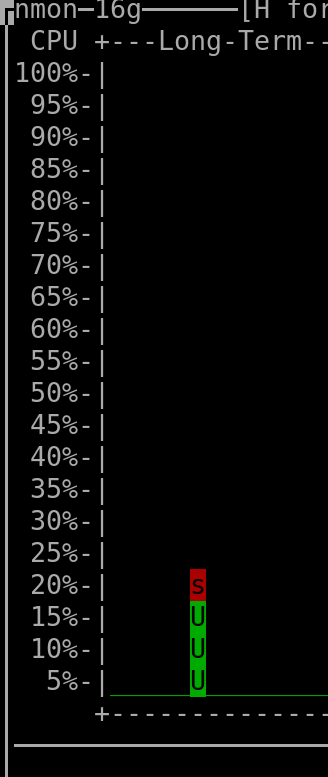	When querying the last 6 hours: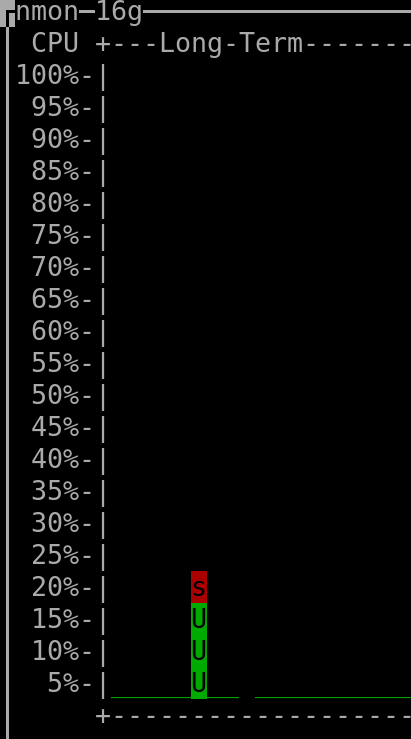	When querying the last 24 hours: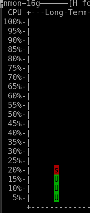
When querying the last 2 days: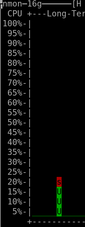	When querying the last 7 days: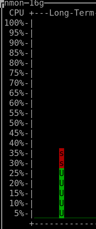	When querying the last 30 days: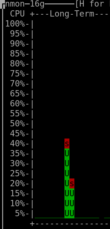
When querying the last 60 days: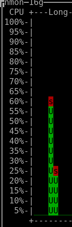	When querying the last 90 days: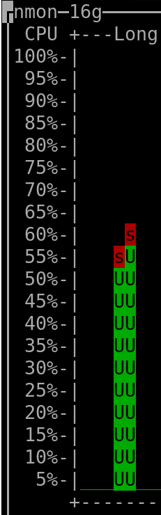	When querying the last 120 days: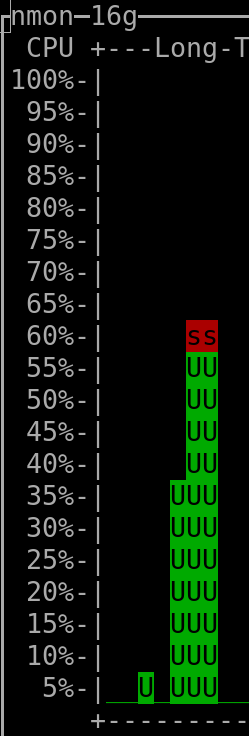
When querying the last 150 days: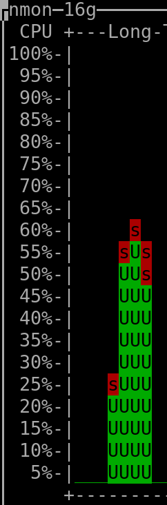	When querying the last 180 days: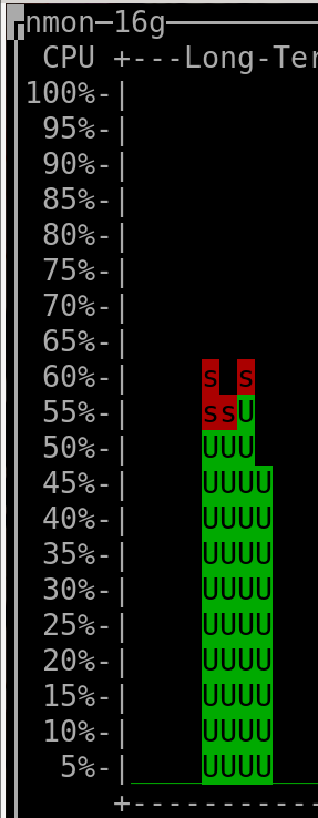	When querying the last 210 days: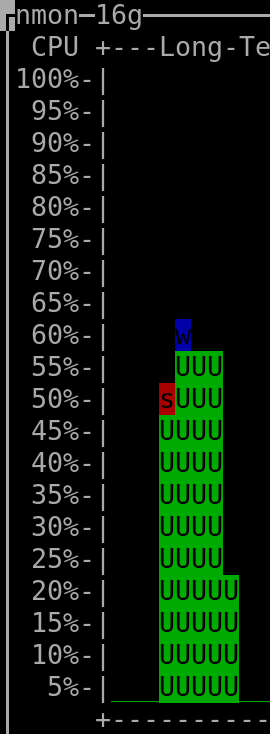
When querying the last 240 days: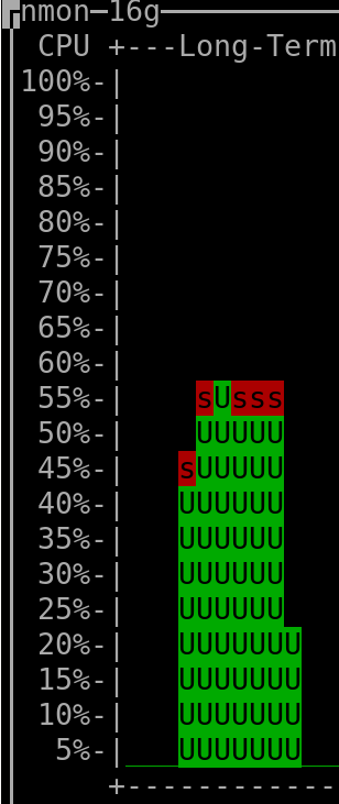	When querying the last 270 days: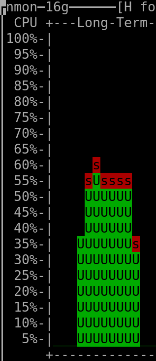	When querying the last 300 days: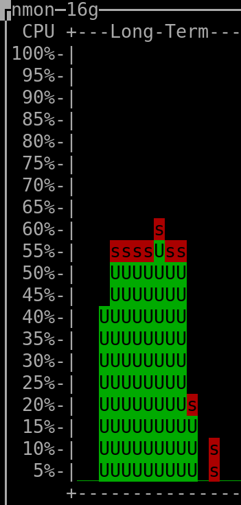
When querying the last 330 days: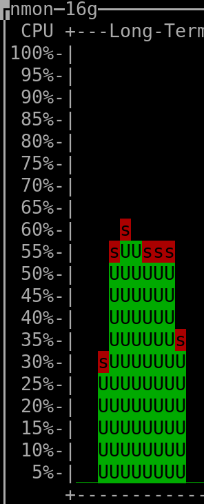

(output generated by "nmon" and then keyboard keys "l" and "-")

The CPU installed on the host was "Intel(R) Xeon(R) CPU E3-1271 v3 @ 3.60GHz".
(the vCPUs allocated to the VM hosting Clickhouse were 4, but irrelevant as this measurement was taken on the server that hosted all the VMs => it therefore encompasses everything, as mentioned above)
The amount of RAM used by the Clickhouse-DB in the VM was so far ~400MiB at rest ("RES"-column of "htop"), spiking to ~600MiB when a refresh of dashboard was triggered.
The VM hosting Clickhouse had 4Gib RAM available and 4 vCPUs (KVM).
The total amount of rows/datapoints queried in the DB when checking the above shown CPU consumption for the 30 days timerange was ~8.1 million (~90 metrics * ~90'000 datapoints per metric).
The total amount of rows present in the Clickhouse database was ~90 million (I'm currently not using most of the metrics that are being gathered - what shall I say, better too much than to miss something by mistake, hehe).
The total used storage space (including not yet deleted "parts" that were already merged into higher-level "parts") used by Clickhouse (to store a bit more than ~30 days worth of data for all metrics, which are in total ~90 million rows) is 260MiB => multiplied for 3 years it should result in ~9.4GiB (or less), which is absolutely ok for me, especially if compared to the ~40GiB that I needed previously when using Carbon&Graphite&Whisper to hold data for only 2 years
The storage used by the Clickhouse-DB in the VM is not local but linked to the host's 9p-mount.

This graph shows the write-activity before & after I deactivated Carbon&Graphite&Whisper (and left only Clickhouse running - before that point both were running):

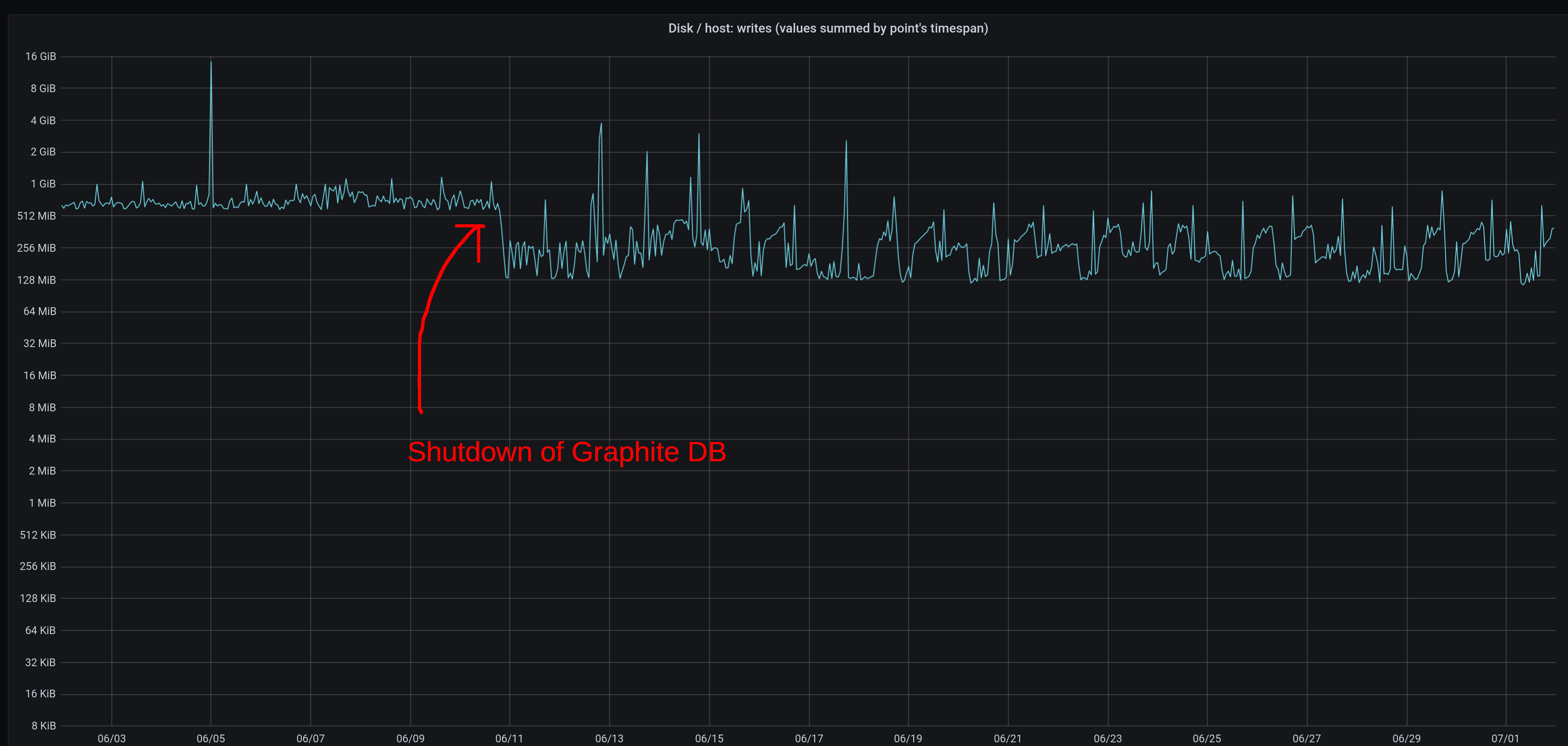
(keep in mind that the chart shows the summed write-activity within a 30-minutes timespan per pixel - it's not some sort of average)
Not a lot of difference (the chart on the Y-axis is logarithmic) but I personally like more the fluctuations of Clickhouse than the everlasting constant write activity of Graphite (it always gave me the impression that other processes were never ever able to achieve their max I/O rate).
The write activity of Clickhouse will increase a little bit in the future because of my personal decision to partition tables by year (instead of by month), therefore from time to time the DB will create single big/very_big "parts" (of a higher level) to get rid of multiple smaller "parts" (of a lower level).
If you're not familiar with Clickhouse you're now probably thinking about a linear increase, but that would be wrong - the higher the level of the aggregation the less frequently it will happen => the write-curve will increase, but it will gradually flatten because of the decreasing frequency (that's at least what I hope will happen, hehe).

If you aren't familiar with the Clickhouse DB, this chart shows you quite well its typical behaviour:
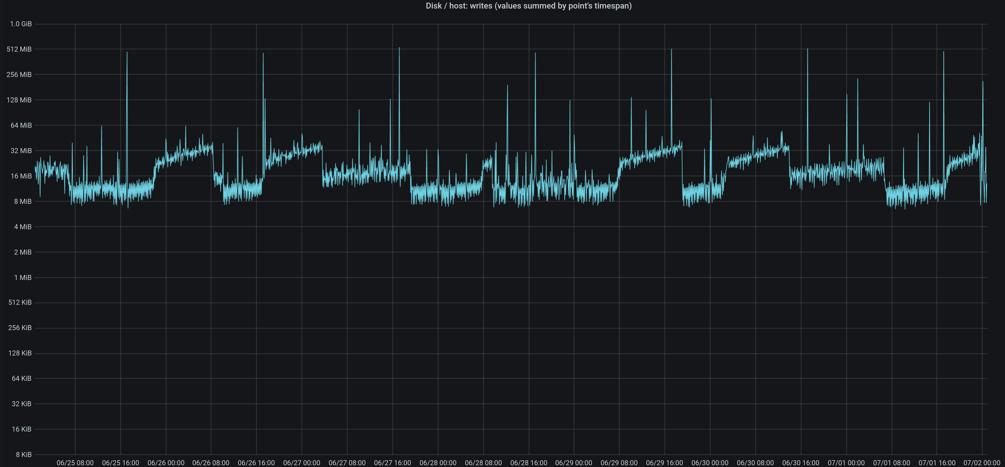
chart showing gradually increasing write-rates, to then suddenly drop to then gradually increase again, etc...
The DB keeps creating low-level files for each bundle of new incoming data (delivered by the "Collectd" agents and inserted into the "buffered"-table).
Once a certain amount of low-level files/"parts" exist, it will read all their contents to then create a file/"part" of a higher level.
Then the whole thing starts over again (but depending on the amount of files/"parts" that you have + their size + their level, the DB might decide for a little while to integrate the brand new rows very quickly into the higher-level-aggregated files/"parts" without going through intermediate levels), and so on.
All this will therefore create over time "waves" of increasing write activity, with sudden drops once the DB thinks that the higher-level files are big enough and that it should focus again on creating only lower-level files/"parts" without touching the higher-level ones.

In Clickhouse you can check about in/active parts/files of a table with this query:

select table, partition, active, level, count(*), sum(data_compressed_bytes)
from system.parts
where database = 'health_metrics'
and table in ('collectd_metrics')
/*and active = 1*/
group by table, partition, active, level
order by table asc, partition, active desc, level

Ongoing/active "merges" of lower-level "parts" into higher-level "parts" can be checked with this query:

SELECT database,table,elapsed,round(progress,4),num_parts,result_part_name,total_size_bytes_compressed, memory_usage
from system.merges

Useful Clickhouse utilities are listed here.
"chproxy" is especially useful if you want/have to limit the amount of concurrent requests sent to Clickhouse (e.g. if you have a big Dashboard with many charts that execute many SQLs that stress your DB, or many users that might potentially trigger refreshes of their dashboards at the same time).

I set in my virt-manager the host's filesystem's share (the one used by my Clickhouse-DB) as follows:

Type: mount
Driver: Path
Mode: Mapped
Write policy: Immediate

By using these settings I do not have any problems related to file-ownershipt/permissions.
I got problems when trying to mount the host's shared filesystem while the VMs were being booted (trying to mount before the network becomes available) => got fixed by specifying the "_netdev"-option in fstab (shown below.
Performance was really bad with 9p when not using the "msize"-setting shown below (as recommended in some forums - I personally have no clue about how the 9p-protocol works).
Summarized, what I'm using now in fstab is:

9p_clickhouse_share    /opt/mysubdir/my_clickhouse_dedicated_dir        9p      noatime,trans=virtio,msize=262144,version=9p2000.L,_netdev    0 0

That's it.

7- Downloads

As, even by having the 3 SQL-templates/examples shown above you might not want to write all the rest on your own or you might want more examples, here are the ones that I'm currently using for my own dashboard.

8- Changelog

03.Jul.2020 - 09.Jul.2020: formatting changes.
10.Jul.2020: created "Downloads" chapter and added SQLs for Grafana/Clickhouse
11.Jul.2020: multiple edits, beautifications, corrections => article is now in its final state => future updates will focus on added informations and/or corrections for published results.
31.Jul.2020: added to chapter 6 the chart of CPU usage for 60-days query.
13.Sep.2020: added to chapter 6 the chart of CPU usage for 90-days query.
16.Oct.2020: added to chapter 6 the chart of CPU usage for 120-days query.
Additional details:
The database table currently contains a total of 384 million rows. Those rows are currently distributed over 7 active "parts" having a size of 20KiB, 1MiB, 4MiB, 5MiB, 50MiB, 60MiB, 105MiB, the total used disk space purely by the data being therefore about 230MiB.
A test done using a separate table (transferred all rows into the test-table) shows that the savings of merging the 7 separate "parts" (by executing "optimize table xxx final") would be of only 1MB (expected as row order is already very good, therefore compression algos are already working very well); CPU usage might show some improvement after such a "merge" as data from less "parts" would have to be queried&merged but so far I'll just let it be as current performance is good enough.
The total amount of storage used by all Clickhouse datafiles on the filesystem (includes therefore overhead like indexes and checksums) is 256MiB.
19.Nov.2020: added to chapter 6 the chart of CPU usage for 150-days query.
Remark: upgrading the Linux kernel (from 4.14.x to 5.4.x) and adding a new network interface (Wireguard VPN) added in Nov.2020 automatically 30 metrics being monitored by Collectd and sent to the DB, of which 18 are then as well queried when refreshing the dashboard (in addition to what was queried up to until Oct.2020).
14.Dec.2020: added to chapter 6 the chart of CPU usage for 180-days query.
The database table is currently 300MiB big (1 "part" of 248MBs + 1 "part" of 42MBs + 7 additional very small "parts" for the remaining 10MBs) and contains a total of 550M rows.
17.Jan.2021: added to chapter 6 the chart of CPU usage for 210-days query.
The Clickhouse DB successfully created the new partition for 2021. The partition containing 2020-data currently holds 4 active "parts" => I will check during the next months if they'll get automatically merged into fewer ones or even a single one.
Current total amount of rows is 644M, total used compressed storage is 347MiB (total uncompressed amount of bytes saved is 36GiB).
15.Feb.2021: added to chapter 6 the chart of CPU usage for 240-days query.
Peak RAM usage by Clickhouse process during the refresh was ~580MiB.
17.Mar.2021: added to chapter 6 the chart of CPU usage for 270-days query.
Nothing special going on - data still split into 2 partitions, old 2020-partition still has the same 4 "parts" mentioned above, the 2021-partition has currently on average 6 "parts" (1x 65MiB, 1x 21MiB, 3x ~7MiB each).
16.Apr.2021: added to chapter 7 the chart of CPU usage for 300-days query.
Peak RAM usage by Clickhouse process during the refresh was ~560MiB
18.May.2021: added to chapter 7 the chart of CPU usage for 330-days query.
Current total amount of rows is 985M, total used compressed storage is 508MiB (total uncompressed amount of bytes saved is 55GiB).